1 Introduction

1.1 Time Series Forecasting

Time series forecasting, or time series prediction, takes an existing series of data and forecasts the data values. The goal is to observe or model the existing data series to enable future unknown data values to be forecasted accurately. Examples of data series include financial data series (stocks, indices, rates, etc.), physically observed data series (sunspots, weather, etc.), and mathematical data series (Fibonacci sequence, integrals of differential equations, etc.). The phrase “time series” generically refers to any data series, whether or not the data are dependent on a certain time increment.

Throughout the literature, many techniques have been implemented to perform time series forecasting. This paper will focus on two techniques: neural networks and k-nearest-neighbor. This paper will attempt to fill a gap in the abundant neural network time series forecasting literature, where testing arbitrary neural networks on arbitrarily complex data series is common, but not very enlightening. This paper thoroughly analyzes the responses of specific neural network configurations to artificial data series, where each data series has a specific characteristic. A better understanding of what causes the basic neural network to become an inadequate forecasting technique will be gained. In addition, the influence of data preprocessing will be noted. The forecasting performance of k-nearest-neighbor, which is a much simpler forecasting technique, will be compared to the neural networks’ performance. Finally, both techniques will be used to forecast a real data series.

Difficulties inherent in time series forecasting and the importance of time series forecasting are presented next. Then, neural networks and k-nearest-neighbor are detailed. Section 2 presents related work. Section 3 gives an application level description of the test-bed application, and Section 4 presents an empirical evaluation of the results obtained with the application.

1.1.1 Difficulties

Several difficulties can arise when performing time series forecasting. Depending on the type of data series, a particular difficulty may or may not exist. A first difficulty is a limited quantity of data. With data series that are observed, limited data may be the foremost difficulty. For example, given a company’s stock that has been publicly traded for one year, a very limited amount of data are available for use by the forecasting technique.

A second difficulty is noise. Two types of noisy data are (1) erroneous data points and (2) components that obscure the underlying form of the data series. Two examples of erroneous data are measurement errors and a change in measurement methods or metrics. In this paper, we will not be concerned about erroneous data points. An example of a component that obscures the underlying form of the data series is an additive high-frequency component. The technique used in this paper to reduce or remove this type of noise is the moving average. The data series becomes after taking a moving average with an interval i of three. Taking a moving average reduces the number of data points in the series by .

A third difficulty is nonstationarity, data that do not have the same statistical properties (e.g., mean and variance) at each point in time. A simple example of a nonstationary series is the Fibonacci sequence: at every step the sequence takes on a new, higher mean value. The technique used in this paper to make a series stationary in the mean is first-differencing. The data series becomes after taking the first-difference. This usually makes a data series stationary in the mean. If not, the second-difference of the series can be taken. Taking the first-difference reduces the number of data points in the series by one.

A fourth difficulty is forecasting technique selection. From statistics to artificial intelligence, there are myriad choices of techniques. One of the simplest techniques is to search a data series for similar past events and use the matches to make a forecast. One of the most complex techniques is to train a model on the series and use the model to make a forecast. K-nearest-neighbor and neural networks are examples of the first and second techniques, respectively.

1.1.2 Importance

Time series forecasting has several important applications. One application is preventing undesirable events by forecasting the event, identifying the circumstances preceding the event, and taking corrective action so the event can be avoided. At the time of this writing, the Federal Reserve Committee is actively raising interest rates to head off a possible inflationary economic period. The Committee possibly uses time series forecasting with many data series to forecast the inflationary period and then acts to alter the future values of the data series.

Another application is forecasting undesirable, yet unavoidable, events to preemptively lessen their impact. At the time of this writing, the sun’s cycle of storms, called solar maximum, is of concern because the storms cause technological disruptions on Earth. The sunspots data series, which is data counting dark patches on the sun and is related to the solar storms, shows an eleven-year cycle of solar maximum activity, and if accurately modeled, can forecast the severity of future activity. While solar activity is unavoidable, its impact can be lessened with appropriate forecasting and proactive action.

Finally, many people, primarily in the financial markets, would like to profit from time series forecasting. Whether this is viable is most likely a never-to-be-resolved question. Nevertheless many products are available for financial forecasting.

1.2 Neural Networks

1.2.1 Background

A neural network is a computational model that is loosely based on the neuron cell structure of the biological nervous system. Given a training set of data, the neural network can learn the data with a learning algorithm; in this research, the most common algorithm, backpropagation, is used. Through backpropagation, the neural network forms a mapping between inputs and desired outputs from the training set by altering weighted connections within the network.

A brief history of neural networks follows[1]. The origin of neural networks dates back to the 1940s. McCulloch and Pitts (1943) and Hebb (1949) researched networks of simple computing devices that could model neurological activity and learning within these networks, respectively. Later, the work of Rosenblatt (1962) focused on computational ability in perceptrons, or single-layer feed-forward networks. Proofs showing that perceptrons, trained with the Perceptron Rule on linearly separable pattern class data, could correctly separate the classes generated excitement among researchers and practitioners.

This excitement waned with the discouraging analysis of perceptrons presented by Minsky and Papert (1969). The analysis pointed out that perceptrons could not learn the class of linearly inseparable functions. It also stated that the limitations could be resolved if networks contained more than one layer, but that no effective training algorithm for multi-layer networks was available. Rumelhart, Hinton, and Williams (1986) revived interest in neural networks by introducing the generalized delta rule for learning by backpropagation, which is today the most commonly used training algorithm for multi-layer networks.

More complex network types, alternative training algorithms involving network growth and pruning, and an increasing number of application areas characterize the state-of-the-art in neural networks. But no advancement beyond feed-forward neural networks trained with backpropagation has revolutionized the field. Therefore, much work still waits.

1.2.2 Feed-Forward Neural Networks

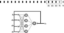
Figure 1.1 depicts an example feed-forward neural network. A neural network can have any number of layers, units per layer, network inputs, and network outputs. This network has four units in the first layer (layer A) and three units in the second layer (layer B), which are called hidden layers. This network has one unit in the third layer (layer C), which is called the output layer. Finally, this network has four network inputs and one network output. Some texts consider the network inputs to be an additional layer, the input layer, but since the network inputs do not implement any of the functionality of a unit, the network inputs will not be considered a layer in this discussion.

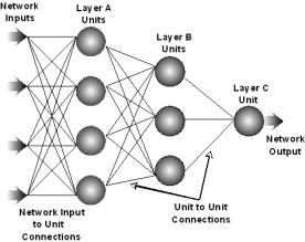
Figure 1.1 A three-layer feed-forward neural network.

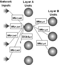
Figure 1.2 Unit with its weights and bias.

If a unit is in the first layer, it has the same number of inputs as there are network inputs; if a unit is in succeeding layers, it has the same number of inputs as the number of units in the preceding layer. Each network-input-to-unit and unit-to-unit connection (the lines in Figure 1.1) is modified by a weight. In addition, each unit has an extra input that is assumed to have a constant value of one. The weight that modifies this extra input is called the bias. All data propagate along the connections in the direction from the network inputs to the network outputs, hence the term feed-forward. Figure 1.2 shows an example unit with its weights and bias and with all other network connections omitted for clarity.

In this section and the next, subscripts c, p, and n will identify units in the current layer, the previous layer, and the next layer, respectively. When the network is run, each hidden layer unit performs the calculation in Equation 1.1 on its inputs and transfers the result (O_c) to the next layer of units.

Equation 1.1 Activation function of a hidden layer unit.

O_c is the output of the current hidden layer unit c, P is either the number of units in the previous hidden layer or number of network inputs, i_c,p is an input to unit c from either the previous hidden layer unit p or network input p, w_c,p is the weight modifying the connection from either unit p to unit c or from input p to unit c, and b_c is the bias.

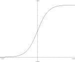
In Equation 1.1, h_Hidden(x) is the sigmoid activation function of the unit and is charted in Figure 1.3. Other types of activation functions exist, but the sigmoid was implemented for this research. To avoid saturating the activation function, which makes training the network difficult, the training data must be scaled appropriately. Similarly, before training, the weights and biases are initialized to appropriately scaled values.

Figure 1.3 Sigmoid activation function. Chart limits are x=±7 and y=-0.1, 1.1.

Each output layer unit performs the calculation in Equation 1.2 on its inputs and transfers the result (O_c) to a network output.

Equation 1.2 Activation function of an output layer unit.

O_c is the output of the current output layer unit c, P is the number of units in the previous hidden layer, i_c,p is an input to unit c from the previous hidden layer unit p, w_c,p is the weight modifying the connection from unit p to unit c, and b_c is the bias. For this research, h_Output(x) is a linear activation function[2].

1.2.3 Backpropagation Training

To make meaningful forecasts, the neural network has to be trained on an appropriate data series. Examples in the form of <input, output> pairs are extracted from the data series, where input and output are vectors equal in size to the number of network inputs and outputs, respectively. Then, for every example, backpropagation training[3] consists of three steps:

1. Present an example’s input vector to the network inputs and run the network: compute activation functions sequentially forward from the first hidden layer to the output layer (referencing Figure 1.1, from layer A to layer C).

2. Compute the difference between the desired output for that example, output, and the actual network output (output of unit(s) in the output layer). Propagate the error sequentially backward from the output layer to the first hidden layer (referencing Figure 1.1, from layer C to layer A).

3. For every connection, change the weight modifying that connection in proportion to the error.

When these three steps have been performed for every example from the data series, one epoch has occurred. Training usually lasts thousands of epochs, possibly until a predetermined maximum number of epochs (epochs limit) is reached or the network output error (error limit) falls below an acceptable threshold. Training can be time-consuming, depending on the network size, number of examples, epochs limit, and error limit.

Each of the three steps will now be detailed. In the first step, an input vector is presented to the network inputs, then for each layer starting with the first hidden layer and for each unit in that layer, compute the output of the unit’s activation function (Equation 1.1 or Equation 1.2). Eventually, the network will propagate values through all units to the network output(s).

In the second step, for each layer starting with the output layer and for each unit in that layer, an error term is computed. For each unit in the output layer, the error term in Equation 1.3 is computed.

Equation 1.3 Error term for an output layer unit.

D_c is the desired network output (from the output vector) corresponding to the current output layer unit, O_c is the actual network output corresponding to the current output layer unit, and is the derivative of the output unit linear activation function, i.e. 1. For each unit in the hidden layers, the error term in Equation 1.4 is computed.

Equation 1.4 Error term for a hidden layer unit.

N is the number of units in the next layer (either another hidden layer or the output layer), d_n is the error term for a unit in the next layer, and w_n,c is the weight modifying the connection from unit c to unit n. The derivative of the hidden unit sigmoid activation function, , is .

In the third step, for each connection, Equation 1.5, which is the change in the weight modifying that connection, is computed and added to the weight.

Equation 1.5 Change in the weight modifying the connection from unit p or network input p to unit c.

The weight modifying the connection from unit p or network input p to unit c is w_c,p, a is the learning rate (discussed later), and O_p is the output of unit p or the network input p. Therefore, after step three, most, if not all weights will have a different value. Changing weights after each example is presented to the network is called on-line training. Another option, which is not used in this research, is batch training, where changes are accumulated and applied only after the network has seen all examples.

The goal of backpropagation training is to converge to a near-optimal solution based on the total squared error calculated in Equation 1.6.

Equation 1.6 Total squared error for all units in the output layer.

Uppercase C is the number of units in the output layer, D_c is the desired network output (from the output vector) corresponding to the current output layer unit, and O_c is the actual network output corresponding to the current output layer unit. The constant ½ is used in the derivation of backpropagation and may or may not be included in the total squared error calculation. Referencing Equation 1.5, the learning rate controls how quickly and how finely the network converges to a particular solution. Values for the learning rate may range from 0.01 to 0.3.

1.2.4 Data Series Partitioning

One typical method for training a network is to first partition the data series into three disjoint sets: the training set, the validation set, and the test set. The network is trained (e.g., with backpropagation) directly on the training set, its generalization ability is monitored on the validation set, and its ability to forecast is measured on the test set. A network’s generalization ability indirectly measures how well the network can deal with unforeseen inputs, in other words, inputs on which it was not trained. A network that produces high forecasting error on unforeseen inputs, but low error on training inputs, is said to have overfit the training data. Overfitting occurs when the network is blindly trained to a minimum in the total squared error based on the training set. A network that has overfit the training data is said to have poor generalization ability.

To control overfitting, the following procedure to train the network is often used:

1. After every n epochs, sum the total squared error for all examples from the training set (i.e., where uppercase X is the number of examples in the training set and E_C is from Equation 1.6).

2. Also, sum the total squared error for all examples from the validation set. This error is the validation error.

3. Stop training when the trend in the error from step 1 is downward and the trend in the validation error from step 2 is upward.

When consistently the error in step 2 increases, while the error in step 1 decreases, this indicates the network has over-learned or overfitted the data and training should stop.

When using real-world data that is observed (instead of artificially generated), it may be difficult or impossible to partition the data series into three disjoint sets. The reason for this is the data series may be limited in length and/or may exhibit nonstationary behavior for data too far in the past (i.e., data previous to a certain point are not representative of the current trend).

1.3 K-Nearest-Neighbor

In contrast to the complexity of the neural network forecasting technique, the simpler k-nearest-neighbor forecasting technique is also implemented and tested. K-nearest-neighbor is simpler because there is no model to train on the data series. Instead, the data series is searched for situations similar to the current one each time a forecast needs to be made.

To make the k-nearest-neighbor process description easier, several terms will be defined. The final data points of the data series are the reference, and the length of the reference is the window size. The data series without the last data point is the shortened data series. To forecast the data series’ next data point, the reference is compared to the first group of data points in the shortened data series, called a candidate, and an error is computed. Then the reference is moved one data point forward to the next candidate and another error is computed, and so on. All errors are stored and sorted. The smallest k errors correspond to the k candidates that closest match the reference. Finally, the forecast will be the average of the k data points that follow these candidates. Then, to forecast the next data point, the process is repeated with the previously forecasted data point appended to the end of the data series. This can be iteratively repeated to forecast n data points.

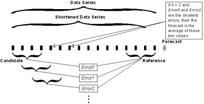
Figure 1.4 K-nearest-neighbor forecasting with window size of four and k=2.

2 Related Work

Perhaps the most influential paper on this research was Drossu and Obradovic (1996). The authors investigate a hybrid stochastic and neural network approach to time series forecasting, where first an appropriate autoregressive model of order p is fitted to a data series, then a feed-forward neural network with p inputs is trained on the series. The advantage to this method is that the autoregressive model provides a starting point for neural network architecture selection. In addition, several other topics pertinent to this research are presented. The authors use real-world data series in the evaluation, but there is one deficiency in their method: their forecasts are compared to data that were part of the validation set, and therefore in-sample, which does not yield an accurate error estimate. This topic is covered in more detail in Section 3.1.1 of this paper.

Zhang and Thearling (1994) present another empirical evaluation of time series forecasting techniques, specifically feed-forward neural networks and memory-based reasoning, which is a form of k-nearest-neighbor search. The authors show the effects of varying several neural network and memory-based reasoning parameters in the context of a real-world data set used in a time series forecasting competition. The main contribution of this paper is its discussion of parallel implementations of the forecasting techniques, which dramatically increase the data processing capabilities. Unfortunately, the results presented in the paper are marred by typographical errors and omissions.

Geva (1998) presents a more complex technique of time series forecasting. The author uses the multiscale fast wavelet transform to decompose the data series into scales, which are then fed through an array of feed-forward neural networks. The networks’ outputs are fed into another network, which then produces the forecast. The wavelet transform is an advanced, relatively new technique and is presented in some detail in the paper. The author does a good job of baselining the wavelet network’s favorable performance with other published results, thereby justifying further research. This is definitely an important future research direction. For a thorough discussion of wavelet analysis of time series, see Torrence and Compo (1998).

Another more complex approach to time series forecasting can be found in Lawrence, Tsoi, and Giles (1996). The authors develop an intelligent system to forecast the direction of change of the next value of a foreign exchange rate time series. The system preprocesses the time-series, encodes the series with a self-organizing map, feeds the output of the map into a recurrent neural network for training, and uses the network to make forecasts. As a secondary step, after training the network is analyzed to extract the underlying deterministic finite state automaton. The authors also thoroughly discuss other issues relevant to time series forecasting.

Finally, Kingdon (1997) presents yet another complex approach to time series forecasting—specifically financial forecasting. The author’s goal is to present and evaluate an automated intelligent system for financial forecasting that utilizes neural networks and genetic algorithms. Because this is a book, extensive history, background information, and theory is presented with the actual research, methods, and results. Both neural networks and genetic algorithms are detailed prior to discussing the actual system. Then, a complete application of the system to an example data series is presented.

3 Application Level - Forecaster

To test various aspects of feed-forward neural network design, training, and forecasting, as well as k-nearest-neighbor forecasting, a test-bed Microsoft Windows application termed Forecaster was written. Various neural network applications are available for download on the Web, but for the purposes of this research, an easily modifiable and upgradeable application was desired. Also, coding the various algorithms and techniques is, in this author’s opinion, the best way to learn them. Forecaster is written in C++ using Microsoft Visual C++ 6.0 with the Microsoft Foundation Classes (MFC). To make the application extensible and reusable, object-oriented analysis and design was performed whenever applicable. A class-level description of Forecaster is given in Appendix A. In addition to fulfilling the needs of this research, Forecaster is intended to eventually be a useful tool for problems beyond time series forecasting.

3.1 Neural Networks

3.1.1 Data Parsing

There are two types of data on which a neural network can be trained: time series data and classification data. Examples of time series data were given in Section 1.1. In contrast, classification data consist of n-tuples, where there are m attributes that are the network inputs and classifications that are the network outputs[4]. Forecaster parses time series data from a single column of newline-separated values within a text file (*.txt). Forecaster parses classification data from multiple columns of comma-separated values within a comma-separated-values text file (*.csv).

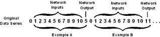
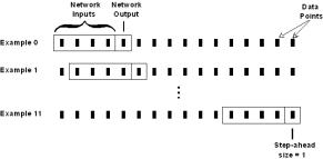
To create the examples in the form of <input, output> pairs referenced in Section 1.2.3, first Forecaster parses the time series data from the file into a one-dimensional array. Second, any preprocessing the user has specified in the Neural Network Wizard (discussed in Section 3.1.3) is applied. Third, as shown in Figure 3.1, a moving window is used to create the examples, in this case for a network with four inputs and one output.

In Figure 3.1 (a), the network will be trained to forecast one step ahead (a step-ahead size of one). When a forecast is made, the user can specify a forecast horizon, which is the number of data points forecasted, greater than or equal to one. 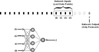In this case, a forecast horizon greater than one is called iterative forecasting—the network forecasts one step ahead, and then uses that forecast to forecast another step ahead, and so on. Figure 3.2 shows iterative forecasting. Note that the process shown in Figure 3.2 can be continued indefinitely.

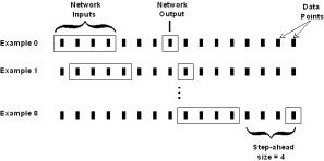
In Figure 3.1 (b), the network will be trained to forecast four steps ahead. If the network is trained to forecast n steps ahead, where , then when a forecast is made, the user can only make one forecast n steps ahead. This is called direct forecasting and is shown in Figure 3.3 for four steps ahead. Note that the number of examples is reduced by .

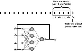
In Figure 3.2 and Figure 3.3, the last data points, saved for forecasting to seed the network inputs, are the last data points within either the training set or validation set, depending on which set is “closer” to the end of the data series. By seeding the network inputs with the last data points, the network is making out-of-sample forecasts. The training set and validation set are considered in-sample, which means the network was trained on them. The training set is clearly in-sample. The validation set is in-sample because the validation error determines when training is stopped (see Section 1.2.4 for more information about validation error).

(a)	(b)
Figure 3.1 Creating examples with a moving window for a network with four inputs and one output. In (a), the step-ahead size is 1; in (b), the step-ahead size is 4.
(a)	(b)
Figure 3.2 Iteratively forecasting (a) the first forecast and (b) the second forecast. This figure corresponds to Figure 3.1 (a).

Figure 3.3 Directly forecasting the only possible data point four steps ahead. This figure corresponds to Figure 3.1 (b).

3.1.2 Neural Network Files

Neural networks can be created and modified with the Neural Network Wizard, which is discussed in more detail in Section 3.1.3. To create a new network, the Wizard can be accessed via the graphical user interface (GUI) in two ways:

· on the menu bar, select NN then New… or

· on the toolbar, click .

The Wizard prompts for a file name, which the neural network will automatically be saved as after training. The extension given to Forecaster neural network files is .fnn.

There are three ways to open an existing Forecaster neural network file:

· on the menu bar, select NN then Open…,

· on the menu bar, select NN then select the file from the most-recently-used list, or

· on the toolbar, click .

Once a network is created or opened, there are two ways to access the Wizard to modify the network:

· on the menu bar, select NN then Modify… or

· on the toolbar, click .

3.1.3 The Wizard

The cornerstone of the application’s GUI is the Neural Network Wizard. The Wizard is a series of dialogs that facilitate the design of a feed-forward neural network. Figure 3.4 (a) through (e) show the five dialogs that make up the Wizard.

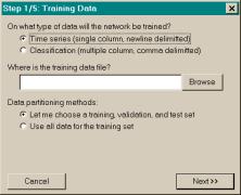
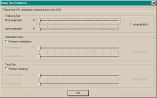
The first dialog, Training Data, enables the user to specify on what type of data the network will be trained, where the data are located, and how the data are to be partitioned. If the user selected Let me choose… in the third field on the Training Data dialog, the Data Set Partition dialog shown in Figure 3.4 (f) appears after the fifth dialog of the Wizard. The Data Set Partition dialog informs the user how many examples are in the data series. The dialog then enables the user to partition the examples into a training set, validation set, and test set. Note that the validation set and test set are optional.

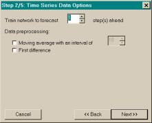
The second dialog, Time Series Data Options, enables the user to set the example step-ahead size, perform a moving average preprocessing, and perform a first-difference preprocessing. If the user had selected Classification… in the Training Data dialog, the Classification Data Options dialog would have appeared instead of the Time Series Data Options dialog. Because classification data are not relevant to this research, the dialog will not be shown or discussed here.

The third dialog, Network Architecture, enables the user to construct the neural network, including specifying the number of network inputs, the number of hidden layers and units per layer, and the number of output layer units. For time series data, the number of output layer units is fixed at one; for classification data, both the number of network inputs and number of output layer units are fixed (depending on information entered in the Classification Data Options dialog). Selecting a suitable number of network inputs for time series forecasting is critical and is discussed in Section 4.2.1. Similarly, selecting the number of hidden layers and units per layer is important and is also discussed in Section 4.2.1.

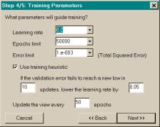
The fourth dialog, Training Parameters, enables the user to control how the network is trained by specifying the learning rate, epochs limit, and error limit. Also, the dialog enables the user to set the parameters for a training heuristic discussed in Section 4.2.2. Finally, the dialog enables the user to adjust the frequency of training information updates for the main application window (the “view”), which also affects the aforementioned training heuristic. The epochs limit parameter provides the upper bound on the number of training epochs; the error limit parameter provides the lower bound on the total squared error given in Equation 1.6. Training stops when the number of epochs grows to the epochs limit or the total squared error drops to the error limit. Typical values for the epochs limit and error limit depend on various factors, including the network architecture and data series. Adjusting the training parameters during training is discussed in Section 3.1.4.

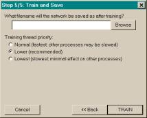
The fifth dialog, Train and Save, enables the user to specify a file name, which the network will be saved as after training. Also, the user can change the priority of the training thread. The training thread performs backpropagation training and is computationally intensive. Setting the priority at Normal makes it difficult for many computers to multi-task. Therefore, it is recommended that the priority be set to Lower or even Lowest for slower computers.

(a)

(b)

(c)

(d)

(e)

(f)

Figure 3.4 The (a) - (e) Neural Network Wizard dialogs and the (f) Data Set Partition dialog. The Wizard dialogs are (a) the Training Data dialog, (b) the Time Series Data Options dialog, (c) the Network Architecture dialog, (d) the Training Parameters dialog, and (e) the Train and Save dialog.

3.1.4 Training

Once the user clicks TRAIN in the Train and Save dialog, the application begins backpropagation training in a new thread. Every n epochs (n is set in the Training Parameters dialog) the main window of the application will display updated information for the current epoch number, total squared error, unscaled error (discussed later in this section), and, if a validation set is created in the Data Set Partition dialog, the validation error. Also, the numbers of examples in the training and validation sets are displayed on the status bar of the window.

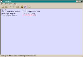
When an error metric value for the currently displayed epoch is less than or equal to the lowest error value reported for that metric during training, the error is displayed in black font. Otherwise, the error is displayed in red font. Figure 3.5 (a) shows a freeze-frame of the application window during training when the validation error is increasing and (b) a freeze-frame after training. Also notice from Figure 3.5 (a) that following each error metric, within parentheses, is the number of view updates since the lowest error value reported for that metric during training.

(a)

(b)

Figure 3.5 Freeze-frames of the application window (a) during training when the validation error is increasing and (b) after training.

To effectively train a neural network, the errors must be monitored during training. Each error value has a specific relation to the training procedure. Total squared error is given in Equation 1.6 and is a common metric for comparing how well different networks learned the same training data set. (Note that the value displayed in the application window does not include the ½ term in Equation 1.6.) But for total squared error to be meaningful, the data set involved in a network comparison must always be scaled equivalently. For example, if data set A is scaled linearly from [0, 1] in trial 1 and is scaled linearly from [-1, 1] in trial 2, comparing the respective total squared errors will be comparing “apples to oranges”. Also, referencing the notation in Equation 1.6, total squared error can be misleading because, depending on the values of D_c and O_c, the value summed may be less than, greater than, or equal to the value of the difference. This is the result of taking the square of the difference.

Unscaled error allows the user to see the actual magnitude of the training set error. “Unscaled” means that the values used to compute the error, which are desired output and actual output, are in the range of the data values in the original, unscaled data series. This is different from total squared error where the values used to compute the error are in the scaled range usable by the neural network (e.g., [0, 1]). Unscaled error is computed in Equation 3.1.

Equation 3.1 Unscaled error for all units in the output layer.

Uppercase C is the number of units in the output layer, UD_c is the unscaled desired network output (from the output vector) corresponding to the current output layer unit, and UO_c is the unscaled actual network output corresponding to the current output layer unit. To eliminate the problem caused by the square in the total squared error, the absolute value of the difference is used instead. An example will highlight the unscaled error’s usefulness: if the unscaled error for an epoch is 50.0 and there are 100 examples in the training data set, then for each example, on average the desired output differs from the network’s actual output by .

If a validation set is created in the Data Set Partition dialog, the validation error can be used to monitor training. The validation error is perhaps the most important error metric and will be used within the training heuristic discussed in Section 4.2.2. Note that if a validation set is not created, the validation error will be 0.0.

The goal of backpropagation training is to find a near-optimal neural network weight-space solution. Local error minima on the training error curve represent sub-optimal solutions that may or may not be the best attainable solution. Therefore, the total squared error, unscaled error, and validation error can be observed, and when an error begins to rise (probably after consistently dropping for thousands of epochs), the learning rate can be increased to attempt to escape from a local minimum or decreased to find a “finer” solution. A typical increase or decrease is 0.05.

During training, there are two ways to access the Change Training Parameters dialog to change the learning rate, epochs limit, and error limit:

· on the menu bar, select NN then Change Training Parameters… or

· on the toolbar, click .

Note that the epochs limit and error limit can be changed if they were set too low or too high.

There are two ways to immediately stop training:

· on the menu bar, select NN then Stop Training or

· on the toolbar, click .

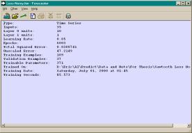
After a network is trained, information about the network will be displayed in the main application window. If desired, this information can be saved to a text file in two ways:

· on the menu bar, select NN then Save to Text File… or

· on the toolbar, click .

To view a simple chart of the data series on which the network was trained, on the menu bar, select View then Training Data Chart….

3.1.5 Forecasting

After a network is trained, a forecast can be made. Figure 3.6 shows the Time Series Forecasting dialog. The dialog can be accessed in two ways:

· on the menu bar, select NN then Start a Forecast… or

· on the toolbar, click .

The dialog informs the user for which kind of forecasting the network was trained, either iterative or direct. If the network was trained for iterative forecasting, the user can specify how many steps ahead the network should iteratively forecast. Otherwise, if the network was trained for direct forecasting n steps ahead, the user can make only one forecast n steps ahead. The dialog also enables the user to enter an optional forecast output file. Finally, the forecast list box will show the forecasts.

After a forecast is made, a simple chart of the forecast can be viewed: on the menu bar, select View then Forecast Data Chart…. If the user specified in the Time Series Data Options dialog that the network should train on the first-difference of the data series, Forecaster automatically reconstitutes the data series, and shows the actual values in the forecast list box, output file, and the forecast data chart—not first-difference values. In contrast, the first-difference values on which the network was trained are shown in the training data chart.

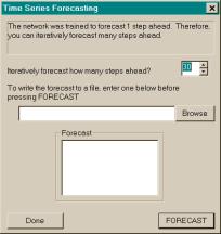
Figure 3.6 Neural network Time Series Forecasting dialog.

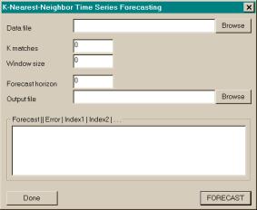
Figure 3.7 K-Nearest-Neighbor Time Series Forecasting dialog.

3.2 K-Nearest-Neighbor

The dialog to perform a k-nearest-neighbor forecast, shown in Figure 3.7, can be accessed via the menu bar: select Other then K-Nearest-Neighbor…. The dialog enables the user to enter the name of the data file that will be searched, the number of k matches, the window size, the forecast horizon, and an optional output file. Values for the number of k matches and window size depend on the data series to be forecast. Note that the forecast list box shows not only the forecast, but also the average error for that forecast data point and the zero-based indices of the k matches.

4 Empirical Evaluation

4.1 Data Series

The goal of the following evaluation is to determine the neural network’s response to various changes in the data series given a feed-forward neural network and starting with a relatively simple artificially generated data series. The evaluation is intended to reveal characteristics of data series that adversely affect neural network forecasting. Note that the conclusions drawn may be specific to these data series and not generally applicable. Unfortunately this is the rule in neural networks as they are more art than science! For comparison, the simpler k-nearest-neighbor forecasting technique will also be applied to the data series. Finally, neural networks and k-nearest-neighbor will be applied to forecast a real-world data series.

The base artificially generated data series is a periodic “sawtooth” wave, shown in Figure 4.1 (a). This data series was chosen because it is relatively simple but not trivial, has smooth segments followed by sharp transitions, and is stationary in the mean. Herein it will be referred to as the “original” data series. Three periods are shown in Figure 4.1 (a), and there are seventy-two data points per period. The actual data point values for a period are: 0, 1, 2, …, 9, 10, 5, 0, 1, 2, …, 19, 20, 15, 10, 5, 0, 1, 2, …, 29, 30, 25, 20, 15, 10, 5.

By adding Gaussian (normal) random noise to the original data series, the second data series is created, termed “less noisy” (less noisy than the third data series), and is shown in Figure 4.1 (b). This series was chosen because it contains a real-world difficulty in time series forecasting: a noisy component that obscures the underlying form of the data series. The less noisy data series has a moderate amount of noise added, but to really obscure the original data series, the third data series contains a significant amount of Gaussian random noise. It is termed “more noisy” and is shown in Figure 4.1 (c). To compare the noise added to the less noisy and more noisy data series, histograms are shown in Figure 4.2. The Gaussian noise used to create the less noisy data series has a mean of zero and a standard deviation of one; the Gaussian noise used to create the more noisy data series has a mean of zero and a standard deviation of three. Microsoft Excel and the Random Number Generation tool under its Tools | Data Analysis… menu was used to create the noisy data series.

To create the fourth data series, the linear function was added to the original. It is termed “ascending” and was chosen because it represents another real-world difficulty in time series forecasting: nonstationarity in the mean. The ascending data series is shown in Figure 4.1 (d).

Finally, the real-world data series chosen is the sunspots data series[5] shown in Figure 4.1 (e). It was chosen because it is a popular series used in the forecasting literature, is somewhat periodic, and is nearly stationary in the mean.

(a)	(b)
(c)	(d)
(e)
Figure 4.1 Data series used to evaluate the neural networks and k-nearest-neighbor: (a) original, (b) less noisy, (c) more noisy, (d) ascending, and (e) sunspots.

(a)	(b)
Figure 4.2 Gaussian random noise added to (a) the less noisy data series and (b) the more noisy data series.

4.2 Neural Network Parameters and Procedure

4.2.1 Architectures

To test how feed-forward neural networks respond to various data series, a network architecture that could accurately learn and model the original series is needed. An understanding of the feed-forward neural network is necessary to specify the number of network inputs. The trained network acts as a function: given a set of inputs it calculates an output. The network does not have any concept of temporal position and cannot distinguish between identical sets of inputs with different actual outputs. For example, referencing the original data series, if there are ten network inputs, among the training examples (assuming the training set covers an entire period) there are several instances where two examples have equivalent input vectors but different output vectors. One such instance is shown in Figure 4.3. This may “confuse” the network during training, and fed that input vector during forecasting, the network’s output may be somewhere in-between the output vectors’ values or simply “way off”!

Figure 4.3 One instance in the original data series where two examples have equivalent input vectors but different output vectors.

Inspection of the original data series reveals that a network with at least twenty-four inputs is required to make unambiguous examples. (Given twenty-three inputs, the largest ambiguous example input vectors would be from zero-based data point 10 to 32 and from 34 to 56.) Curiously, considerably more network inputs are required to make good forecasts, as will be seen in Section 4.4.

Next, through trial-and-error the number of hidden layers was found to be one and the number of units in that layer was found to be ten for the artificial data series. The number of output layer units is necessarily one. This network, called 35:10:1 for shorthand, showed excellent forecasting performance on the original data series, and was selected to be the reference for comparison and evaluation. To highlight any effects of having a too-small or too-large network for the task, two other networks, 35:2:1 and 35:20:1, respectively, are also included in the evaluation. Also, addressing the curiosity raised in the previous paragraph, two more networks, 25:10:1 and 25:20:1, are included.

It is much more difficult to choose the appropriate number of network inputs for the sunspots data series. By inspecting the data series and through trial-and-error, thirty network inputs were selected. Also through trial-and-error, one hidden layer with thirty units was selected. Although this network seems excessively large, it proved to be the best neural network forecaster for the sunspots data series. Other networks that were tried include 10:10:1, 20:10:1, 30:10:1, 10:20:1, 20:20:1, and 30:20:1.

4.2.2 Training

By observing neural network training characteristics, a heuristic algorithm was developed and implemented in Forecaster. The parameters for the heuristic are set within the Training Parameters dialog (see Section 3.1.3). The heuristic requires the user to set the learning rate and epochs limit to higher-than-normal values (e.g., 0.3 and 500,000, respectively) and the error limit to a lower-than-normal value (e.g., ). The heuristic also uses three additional user-set parameters: the number of training epochs before an application window (view) update (update frequency), the number of updates before a learning rate change (change frequency), and a learning rate change decrement (decrement). Finally, the heuristic requires the data series to be partitioned into a training set and validation set. Given these user set parameters, the heuristic algorithm is:

for each view-update during training

if the validation error is higher than the lowest value seen

increment count

if count equals change-frequency

if the learning rate minus decrement is greater than zero

lower the learning rate by decrement

reset count

continue

else

stop training

The purpose of the heuristic is to start with an aggressive learning rate, which will quickly find a coarse solution, and then to gradually decrease the learning rate to find a finer solution. Of course, this could be done manually by observing the validation error and using the Change Training Parameters dialog to alter the learning rate. But an automated solution is preferred, especially for an empirical evaluation.

In the evaluation, the heuristic algorithm is compared to the “simple” method of training where training continues until either the number of epochs grows to the epochs limit or the total squared error drops to the error limit. Networks trained with the heuristic algorithm are termed “heuristically trained”; networks trained with the simple method are termed “simply trained”.

Finally, the data series in Section 4.1 are partitioned so that the training set is the first two periods and the validation set is the third period. Note that “period” is used loosely for less noisy, more noisy, and ascending, since they are not strictly periodic.

4.2.3 Forecasting

The coefficient of determination from Drossu and Obradovic (1996) is used to compare the networks’ forecasting performance and is given in Equation 4.1.

Equation 4.1 Coefficient of determination comparison metric.

The number of data points forecasted is n, x_i is the actual value, is the forecast value, and is the mean of the actual data. The coefficient of determination can have several possible values:

A coefficient of determination close to one is preferable.

To compute the coefficient of determination in the evaluation, the forecasts for the networks trained on the original, less noisy, and more noisy data series are compared to the original data series. This is slightly unorthodox: a forecast from a network trained on one data series, for example, more noisy, is compared to a different data series. But the justification is two-fold. First, it would not be fair to compare a network’s forecast to data that have an added random component. This would be the case if a network was trained and validated on the first three periods of more noisy, and then its forecast was compared to a fourth period of more noisy. Second, the goal of the evaluation is to see what characteristics of data series adversely affect neural network forecasting. In other words, the goal is determining under what circumstances a network can no longer learn the underlying form of the data (generalize), and the underlying form is the original data series. To compute the coefficient of determination for the networks trained on the ascending data series, the ascending series is simply extended. To compute the coefficient of determination for the network trained on the sunspots data series, part of the series is withheld from training and used for forecasting.

4.2.4 Evaluation Specifics

Table 4.1 and Table 4.2 list beginning parameters for all neural networks trained with the heuristic algorithm and simple method, respectively. Parameters for trained networks (e.g., the actual number of training epochs) are presented in Section 4.4 and Section 4.5.

Heuristic Algorithm Training *Update Frequency = 50, Change Frequency = 10, Decrement = 0.05*
Architecture	Learning Rate	Epochs Limit	Error Limit	Data Series O = original L = less noisy M = more noisy A = ascending	Training Set Data Point Range (# of Examples)	Validation Set Data Point Range (# of Examples)
35:20:1	0.3	500,000	1x10^-10	O, L, M, A	0 – 143 (109)	144 – 215 (37)
35:10:1	0.3	500,000	1x10^-10	O, L, M, A	0 – 143 (109)	144 – 215 (37)
35:2:1	0.3	500,000	1x10^-10	O, L, M, A	0 – 143 (109)	144 – 215 (37)
25:20:1	0.3	250,000	1x10^-10	O	0 – 143 (119)	144 – 215 (47)
25:10:1	0.3	250,000	1x10^-10	O	0 – 143 (119)	144 – 215 (47)

Table 4.1 Beginning parameters for heuristically trained neural networks.

Simple Method Training
Architecture	Learning Rate	Epochs Limit	Error Limit	Data Series O = original L = less noisy M = more noisy A = ascending S = sunspots	Training Set Data Point Range (# of Examples)	Validation Set Data Point Range (# of Examples)
35:20:1	0.1	100,000	1x10^-10	O, L, M, A	0 – 143 (109)	144 – 215 (37)
35:10:1	0.1	100,000	1x10^-10	O, L, M, A	0 – 143 (109)	144 – 215 (37)
35:2:1	0.1	100,000	1x10^-10	O, L, M, A	0 – 143 (109)	144 – 215 (37)
30:30:1	0.05	100,000	1x10^-10	S	0 – 165 (136)	-

Table 4.2 Beginning parameters for simply trained neural networks.

Often, two trained networks with identical beginning parameters can produce drastically different forecasts. This is because each network is initialized with random weights and biases prior to training, and during training, networks converge to different minima on the training error curve. Therefore, three candidates of each network configuration were trained. This allows another neural network forecasting technique to be used: forecasting by committee. In forecasting by committee, the forecasts from the three networks are averaged together to produce a new forecast. This may either smooth out noisy forecasts or introduce error from a poorly performing network. The coefficient of determination will be calculated for the three networks’ forecasts and for the committee forecast to determine the best candidate.

4.3 K-Nearest-Neighbor Parameters and Procedure

For k-nearest-neighbor, the window size was chosen based on the discussion of choosing neural network inputs in Section 4.2.1. For the artificially generated series, window size values of 20, 24, and 30 with k=2 are tested. For the sunspots data series, window size values of 10, 20, and 30 with k values of 2 and 3 were tested, but only the best forecasting search, which has a window size of 10 and k=3, will be shown. It is interesting that the best forecasting window size for k-nearest-neighbor on the sunspots data series is 10, but the best forecasting number of neural network inputs is 30. The reason for this difference is unknown. Table 4.3 shows the various parameters for k-nearest-neighbor searches.

K-Matches	Window Size	Data Series O = original L = less noisy M = more noisy S = sunspots	Search Set Data Point Range
2	20	O, L, M	0 – 215
2	24	O, L, M	0 – 215
2	30	O, L, M	0 – 215
3	10	S	0 – 165

Table 4.3 Parameters for k-nearest-neighbor searches.

4.4 Artificial Data Series Results

4.4.1 Heuristically Trained Neural Networks with Thirty-Five Inputs

Figure 4.4 graphically shows the one-period forecasting accuracy for the best candidates for heuristically trained 35:2:1, 35:10:1, and 35:20:1 networks[6]. Figure 4.4 (a), (b), and (c) show forecasts from networks trained on the original, less noisy, and more noisy data series, respectively, and the forecasts are compared to a period of the original data series. Figure 4.4 (d) shows forecasts from networks trained on the ascending data series, and the forecasts are compared to a fourth “period” of the ascending series. For reasons discussed later, in Figure 4.4 (c) and (d) the 35:2:1 network is not included.

Figure 4.5 graphically shows the two-period forecasting accuracy for the best candidates for heuristically trained (a) 35:2:1, 35:10:1, and 35:20:1 networks trained on the less noisy data series and (b) 35:10:1 and 35:20:1 networks trained on the more noisy data series.

Figure 4.6 graphically compares metrics for the best candidates for heuristically trained 35:2:1, 35:10:1, and 35:20:1 networks. Figure 4.6 (a) and (b) compare the number of training epochs and training time[7], respectively, (c) and (d) compare the total squared error and unscaled error, respectively, and (e) compares the coefficient of determination. The vertical axis in (a) through (d) is logarithmic. This is indicative of a wide range in values for each statistic.

Finally, Table 4.4 lists the raw data for the charts in Figure 4.6 and other parameters used in training. For each network configuration, the candidate column indicates which of the three trained candidate networks, or the committee, was chosen as the best based on the coefficient of determination. If the committee was chosen, the parameters and metrics for the best candidate network within the committee are listed. Refer to Table 4.1 for more parameters.

In Figure 4.4 (a), it is clear that the 35:2:1 network is sufficient for making forecasts up to a length of twenty-seven for the original data series, but beyond that, its output is erratic. The forecasts for the 35:10:1 and 35:20:1 networks are near perfect, and are indistinguishable from the original data series. The 35:10:1 and 35:20:1 networks can accurately forecast the original data series indefinitely.

In Figure 4.4 (b), the 35:10:1 and 35:20:1 networks again forecast very accurately, and surprisingly, the 35:2:1 network also forecasts accurately. From Figure 4.6 (a), the 35:2:1 network trained for almost eighteen times more epochs on the original data series than on the less noisy data series. From Figure 4.6 (c) and (d), the 35:2:1 network trained on the less noisy data series has two orders of magnitude higher total squared error and one order higher unscaled error than the 35:2:1 network trained on the original data series. (Remember that the total squared error and unscaled error are computed during training based on the training set.) Despite the higher errors and shorter training time, Figure 4.6 (e) confirms what Figure 4.4 (a) and (b) show: the coefficient of determination for the 35:2:1 network trained on the less noisy data series is significantly better than the 35:2:1 network trained on the original data series.

Perhaps the noisy data kept the 35:2:1 network from overfitting the data series allowing the network to learn the underlying form without learning the noise. This makes sense considering the heuristic algorithm: the algorithm stops training when, despite lowering the learning rate, the validation error stops getting lower. Since the validation error is computed based on the validation set, which has random noise, it makes sense that the validation error would start to rise after only a small number of epochs. This explains the discrepancy in the number of epochs. Therefore, it may be expected that if the 35:2:1 network were trained on the original data series with a similar number of epochs as when it was trained on the less noisy data series (7,250), it too would produce good forecasts. Unfortunately, in other trials this has not shown to be the case.

In Figure 4.4 (c) and (d), the 35:2:1 network is not included because of its poor forecasting performance on the more noisy and ascending data series. Figure 4.6 (e) confirms this. In Figure 4.4 (c), both the 35:10:1 and 35:20:1 networks make decent forecasts until the third “tooth,” when the former undershoots and the latter overshoots the original data series. Comparing the charts in Figure 4.4 (b) and (c) to those in Figure 4.5 (a) and (b), it can be seen that near the end of the first forecasted period many of the forecasts begin diverging or oscillating, which is an indication that the forecast is going awry.

Taking the moving average of the noisy data series would eliminate much of the random noise and would also smooth the sharp peaks and valleys. It is clear from Figure 4.4 (a) that a smoother series is easier to learn (except for the 35:2:1 network), and therefore, if the goal (as it is here) is to learn the underlying form of the data series, it would be advantageous to train and forecast based on the moving average of the noisy data series. But in some data series what appear to be noise may actually be meaningful data, and smoothing this out would be undesirable[8].

In Figure 4.4 (d), the 35:10:1 network does a decent job of forecasting the upward trend, although it adds noisy oscillations. The 35:20:1 network is actually the committee forecast, which is the average of all three 35:20:1-network candidates. This is apparent from its smoothing of the ascending data series. The networks trained on the ascending data series produce long-term forecasts that drop sharply after the first period. This could be a result of the nonstationary mean of the ascending data series.

Taking the first-difference of the ascending data series produces a discontinuous-appearing data series with sharp transitions because the positive slope portions of the series have a slope of 1.1 and the negative slope portions have a slope of –4.9. A neural network heuristically trained on that series was able to forecast the first-difference near perfectly. In this case, it would be advantageous to train and forecast based on the first-difference rather than the ascending data series (especially since Forecaster automatically reconstitutes the forecast from its first-difference).

Finally, by evaluating the charts in Figure 4.6 and data in Table 4.4 some observations can be made:

· Networks train longer (more epochs) on smoother data series like the original and ascending data series.

· The total squared error and unscaled error are higher for noisy data series.

· Neither the number of epochs nor the errors appear to correlate well with the coefficient of determination.

· In most cases, the committee forecast is worse than the best candidate’s forecast. But when the actual values are unavailable for computing the coefficient of determination, choosing the best candidate is difficult. In that situation the committee forecast may be the best choice.

(a)

(b)

(c)

(d)

Figure 4.4 The one-period forecasting accuracy for the best candidates for heuristically trained 35:2:1, 35:10:1, and 35:20:1 networks trained on the (a) original, (b) less noisy, (c) more noisy, and (d) ascending data series.

(a)

(b)

Figure 4.5 The two-period forecasting accuracy for the best candidates for heuristically trained (a) 35:2:1, 35:10:1, and 35:20:1 networks trained on the less noisy data series and (b) 35:10:1 and 35:20:1 networks trained on the more noisy data series.

(a)	(b)
(c)	(d)
(e)
Figure 4.6 Graphical comparison of metrics for the networks in Figure 4.4: (a) epochs, (b) training time, (c) total squared error, (d) unscaled error, and (e) coefficient of determination. Note that the vertical axis is logarithmic for (a) - (d). The raw data are given in Table 4.4.

Arch.	Candidate	Data Series	Ending Learning Rate	Epochs	Total Squared Error	Unscaled Error	Coeff. of Determ. (1 period)	Training Time (sec.)
35:2:1	c	Original	0.05	128850	0.00204144	8.9505	0.0992	127
35:10:1	c	Original	0.05	68095	1.30405e-007	0.0912957	1.0000	193
35:20:1	a	Original	0.05	134524	4.62985e-008	0.0521306	1.0000	694
35:2:1	c	Less Noisy	0.05	7250	0.118615	90.3448	0.8841	7
35:10:1	c	Less Noisy	0.05	3346	0.0271639	44.9237	0.9724	10
35:20:1	b	Less Noisy	0.05	3324	0.0346314	51.1032	0.9226	18
35:2:1	c	More Noisy	0.05	20850	0.429334	223.073	-5.7331	20
35:10:1	c	More Noisy	0.05	3895	0.0788805	101.869	0.2931	11
35:20:1	c	More Noisy	0.05	15624	0.00443201	24.0384	0.0674	81
35:2:1	a	Ascending	0.05	7250	0.0553364	90.7434	-2.4076	7
35:10:1	a	Ascending	0.05	60345	0.00145223	15.8449	0.4851	171
35:20:1	committee (b)	Ascending	0.05	32224	0.00238561	20.9055	0.4430	171

Table 4.4 Parameters and metrics for the networks in Figure 4.4.

4.4.2 Simply Trained Neural Networks with Thirty-Five Inputs

Figure 4.7 graphically shows the one-period forecasting accuracy for the best candidates for simply trained 35:2:1, 35:10:1, and 35:20:1 networks. Figure 4.7 (a), (b), and (c) show forecasts from networks trained on the original, less noisy, and more noisy data series, respectively, and the forecasts are compared to a period of the original data series. Figure 4.7 (d) shows forecasts from networks trained on the ascending data series, and the forecasts are compared to a fourth “period” of the ascending series. In Figure 4.7 (c) the 35:2:1 network is not included.

Figure 4.8 graphically compares metrics for the best candidates for simply trained 35:2:1, 35:10:1, and 35:20:1 networks. Figure 4.8 (a) and (b) compare the total squared error and unscaled error, respectively, and (c) compares the coefficient of determination. The vertical axis in (a) and (b) is logarithmic. The number of epochs and training time are not included in Figure 4.8 because all networks were trained to 100,000 epochs.

Finally, Table 4.5 lists the raw data for the charts in Figure 4.8 and other parameters used in training. Refer to Table 4.2 for more parameters.

In Figure 4.7 (a) the 35:2:1 network forecast is much better than in Figure 4.4 (a). In this case, it seems the heuristic was inappropriate. Notice that the heuristic allowed the 35:2:1 network to train for 28,850 epochs more than the simple method. Also, the total squared error and unscaled error for the heuristically trained network were lower, but so was the coefficient of determination—it was much lower. Again, the forecasts for the 35:10:1 and 35:20:1 networks are near perfect, and are indistinguishable from the original data series.

In Figure 4.7 (b) the 35:2:1 network forecast is worse than in Figure 4.4 (b), whereas the 35:10:1 and 35:20:1 forecasts are about the same as before. Notice that the 35:10:1 forecast is from the committee, but does not appear to smooth the data series’ sharp transitions.

In Figure 4.7 (c), the 35:2:1 network is not included because of its poor forecasting performance on the more noisy data series. The 35:10:1 and 35:20:1 forecasts are slightly worse than before.

In Figure 4.7 (d), the 35:2:1 network is included and its coefficient of determination is much improved from before. The 35:10:1 and 35:20:1 network forecasts are decent, despite the low coefficient of determination for 35:10:1. The forecasts appear to be shifted up when compared to those in Figure 4.4 (d).

Finally, by evaluating the charts in Figure 4.8 and data in Table 4.5 some observations can be made:

· The total squared error and unscaled error are higher for noisy data series with the exception of the 35:10:1 network trained on the more noisy data series. It trained to extremely low errors, orders of magnitude lower than with the heuristic, but its coefficient of determination is also lower. This is probably an indication of overfitting the more noisy data series with simple training, which hurt its forecasting performance.

· The errors do not appear to correlate well with the coefficient of determination.

· In most cases, the committee forecast is worse than the best candidate’s forecast.

· There are four networks whose coefficient of determination is negative, compared with two for the heuristic training method.

(a)

(b)

(c)

(d)

Figure 4.7 The one-period forecasting accuracy for the best candidates for simply trained 35:2:1, 35:10:1, and 35:20:1 networks trained on the (a) original, (b) less noisy, (c) more noisy, and (d) ascending data series.

(a)	(b)
(c)
Figure 4.8 Graphical comparison of metrics for the networks in Figure 4.7: (a) total squared error, (b) unscaled error, and (c) coefficient of determination. Note that the vertical axis is logarithmic for (a) and (b). The raw data are given in Table 4.5.

Arch.	Candidate	Data Series	Ending Learning Rate	Epochs	Total Squared Error	Unscaled Error	Coeff. of Determ. (1 period)	Training Time (sec.)
35:2:1	b	Original	0.1	100000	0.0035864	14.6705	0.9111	99
35:10:1	c	Original	0.1	100000	3.02316e-006	0.386773	1.0000	286
35:20:1	a	Original	0.1	100000	2.15442e-006	0.376312	1.0000	515
35:2:1	b	Less Noisy	0.1	100000	0.0822801	84.8237	0.5201	99
35:10:1	committee (b)	Less Noisy	0.1	100000	0.00341762	17.6535	0.9173	287
35:20:1	b	Less Noisy	0.1	100000	0.00128001	10.8401	0.9453	531
35:2:1	b	More Noisy	0.1	100000	0.360209	203.893	-4.6748	100
35:10:1	a	More Noisy	0.1	100000	2.47609e-009	0.0166514	-0.0056	282
35:20:1	c	More Noisy	0.1	100000	0.000106478	3.65673	-1.5032	519
35:2:1	a	Ascending	0.1	100000	0.023301	59.7174	0.4091	98
35:10:1	a	Ascending	0.1	100000	0.000421792	8.67945	-0.3585	280
35:20:1	b	Ascending	0.1	100000	0.000191954	5.87395	0.4154	529

Table 4.5 Parameters and metrics for the networks in Figure 4.7.

4.4.3 Heuristically Trained Neural Networks with Twenty-Five Inputs

Networks with twenty-five inputs were also tested. According to the analysis presented in Section 4.2.1, twenty-five inputs should be a sufficient number to eliminate any ambiguous examples. Figure 4.9 graphically shows the one-period forecasting accuracy for the best candidates for heuristically trained 25:10:1 and 25:20:1 networks trained on the original data series. Table 4.6 lists the raw data for the parameters and metrics. Refer to Table 4.1 for more parameters.

The forecasting performance for the 25:10:1 and 25:20:1 networks is very poor after the 18^th and 24^th data points, respectively. The networks were heuristically trained, but as can be seen from Table 4.6, the heuristic algorithm never reached a learning rate of 0.05, which is the lowest rate possible given the parameters in Table 4.1. In fact, training was manually stopped at 250,000 epochs, which is significantly more epochs than needed by the 35:10:1 and 35:20:1 networks trained on the original data series in Table 4.4. In other trials, the networks were allowed to train even longer, but the forecasting results were similar to those shown in Figure 4.9. The reason for the poor forecasting is unknown; perhaps the actual number of network inputs needs to be much larger that the number deemed “sufficient”. This serves as a valuable lesson: neural networks are sometimes unpredictable, and a change in architecture or parameters may result in dramatic changes in performance!

Figure 4.9 The one-period forecasting accuracy for the best candidates for heuristically trained 25:10:1 and 25:20:1 networks trained on the original data series.

Arch.

Candidate

Data Series

Ending Learning

Rate

Epochs

Total Squared Error

Unscaled Error

Coeff. of Determ. (1 period)

Training Time (sec.)

25:10:1

committee (b)

Original

0.15

250000

0.0002548

1.87352

-25.4708

651

25:20:1

committee (a)

Original

0.15

250000

9.68947e-005

1.0859

-30.4758

1150

Table 4.6 Parameters and metrics for the networks in Figure 4.9.

4.5 Real-World Data Series Results

The sunspots thirty-four year forecasting accuracy for a simply trained 30:30:1 neural network and k-nearest-neighbor search with k=3 and a window size of 10 is shown graphically in Figure 4.11, and the parameters and metrics for the network and search are listed in Table 4.8 and Table 4.9, respectively. Refer to Table 4.2 and Table 4.3 for more parameters.

Notice from the coefficients of determination that the k-nearest-neighbor once again outperformed the neural network! It is interesting that both methods were able to forecast relatively well the spacing and magnitude of the oscillations in the sunspots data series.

Figure 4.11 Thirty-four year forecasting accuracy for the best candidate simply trained 30:30:1 neural network and k-nearest-neighbor search with k=3 and window size of 10.

Arch.

Candidate

Data Series

Ending Learning

Rate

Epochs

Total Squared Error

Unscaled Error

Coeff. of Determ.

Training Time (sec.)

30:30:1

committee (c)

Sunspots

0.05

100000

5.10651e-005

9.1138

-0.5027

845

Table 4.8 Parameters and metrics for the neural network in Figure 4.11.

K-Matches	Window Size	Data Series	Coeff. of Determ.
3	10	Sunspots	0.2847

Table 4.9 Parameters and coefficient of determination for the k-nearest-neighbor search in Figure 4.11.

5 Conclusion

Section 1 introduced time series forecasting, described the work presented in the typical neural network paper, which justified this paper, and identified several difficulties associated with time series forecasting. Among these difficulties, noisy and nonstationary data were investigated further in this paper. Section 1 also presented feed-forward neural networks and backpropagation training, which was used as the primary time series forecasting technique in this paper. Finally, k-nearest-neighbor was presented as an alternative forecasting technique.

Section 2 briefly discussed previous time series forecasting papers. The most notable of these being the paper by Drossu and Obradovic (1996), who presented compelling research combining stochastic techniques and neural networks. Also of interest were the paper by Geva (1998) and the book by Kingdon (1997), which took significantly more sophisticated approaches to time series forecasting.

Section 3 presented Forecaster and went through several important aspects of its design, including parsing data files, using the Wizard to create networks, training networks, and forecasting using neural networks and k-nearest-neighbor.

Section 4 presented the crux of the paper. First, the data series used in the evaluation were described, and then parameters and procedures used in forecasting were given. Among these was a method for selecting the number of neural network inputs based on data series characteristics (also applicable to selecting the window size for k-nearest-neighbor), a training heuristic, and a metric for making quantitative forecast comparisons. Finally, a variety of charts and tables, accompanied by many empirical observations, were presented for networks trained heuristically and simply and for k-nearest-neighbor.

From these empirical observations several conclusions can be drawn. First, in some cases the heuristic worked better than the simple method and quickly trained a neural network to generalize the underlying form of the data series, without overfitting. In other cases, such as with the 35:2:1 network trained on the original data series, the simple training method produced better results. Unfortunately, one training method does not appear to be clearly better than the other. Second, it appears from the training time and/or error that it is difficult or impossible to determine the network’s forecasting ability. The only way to determine forecasting ability is to make a forecast, compare it to known values, and compute the coefficient of determination. Third, the committee method of forecasting proved better in only a couple of cases. Finally, and most surprisingly, the k-nearest-neighbor forecasting accuracy was consistently better than the neural networks’ forecasting accuracy for the data series tested!

One goal of the research was to determine the performance of various neural network architectures in forecasting various data series. The empirical evaluation showed that increasingly noisy data series increasingly degrade the ability of the neural network to learn the underlying form of the data series and produce good forecasts. Depending on the nature of the data series, taking the moving average may or may not be appropriate to smooth the fluctuations. Nonstationarity in the mean also degraded the network’s forecasting performance. However, training on the first-difference produced better results. Further, a network with too few hidden units, such as 35:2:1, forecasts well on simpler data series, but fails for more complex ones. In contrast, a network with an excessive number of hidden units, such as 35:20:1, appears to do as well as a network with a “sufficient” number of hidden units, such as 35:10:1. Finally, the networks with twenty-five inputs, which should be a sufficient number of inputs, proved to be poor choices for learning even the original data series. All of the above observations add up to one thing: feed-forward neural networks are extremely sensitive to architecture and parameter choices, and making such choices is currently more art than science, more trial-and-error than absolute, more practice than theory.

The field of neural networks is very diverse and opportunities for future research exist in many aspects, including data preprocessing and representation, architecture selection, and application. The future of neural network time series forecasting seems to be in more complex network types that merge other technologies with neural networks, such as wavelet networks. Nevertheless, a theoretic foundation on which to build is absolutely necessary, as more complex networks still suffer from basic problems such as data preprocessing, architecture selection, and parameterization.

6 References

Drossu, R., & Obradovic, Z. (1996). Rapid Design of Neural Networks for Time Series Prediction. IEEE Computational Science & Engineering, Summer 1996, 78-89.

Geva, A. (1998). ScaleNet—Multiscale Neural-Network Architecture for Time Series Prediction. IEEE Transactions on Neural Networks, 9(5), 1471-1482.

Gonzalez, R. C. & Woods, R. E. (1993). Digital Image Processing. New York: Addison-Wesley.

Hebb, D. O. (1949). The Organization of Behavior: A Neuropsychological Theory. New York: Wiley & Sons.

Kingdon, J. (1997). Intelligent Systems and Financial Forecasting. New York: Springer-Verlag.

Lawrence, S., Tsoi, A. C., & Giles, C. L. (1996). Noisy Time Series Prediction Using Symbolic Representation and Recurrent Neural Network Grammatical Inference [Online]. Available: http://www.neci.nj.nec.com/homepages/lawrence/papers/finance-tr96/latex.html [March 27, 2000].

McCulloch, W. S., & Pitts, W. H. (1943). A Logical Calculus of the Ideas Imminent in Nervous Activity. Bulletin of Mathematical Biophysics, 5, 115-133.

Minsky, M., & Papert, S. (1969). Perceptrons: An Introduction to Computational Geometry. Cambridge, MA: MIT Press.

Rosenblatt, F. (1962). Principles of Neurodynamics: Perceptrons and the Theory of Brain Mechanisms. Washington, D. C.: Spartan.

Rumelhart, D. E., Hinton, G. E., & Williams, R. J. (1986). Learning Internal Representations by Error Propagation. In D. E. Rumelhart, et al. (Eds.), Parallel Distributed Processing: Explorations in the Microstructures of Cognition, 1: Foundations, 318-362. Cambridge, MA: MIT Press.

Torrence, C., & Compo, G. P. (1998). A Practical Guide to Wavelet Analysis [Online]. Bulletin of the American Meteorological Society. Available: http://paos.colorado.edu/research/wavelets/ [July 2, 2000].

Zhang, X., & Thearling, K. (1994). Non-Linear Time-Series Prediction by Systematic Data Exploration on a Massively Parallel Computer [Online]. Available: http://www3.shore.net/~kht/text/sfitr/sfitr.htm [March 27, 2000].

Appendix A: Class-level description of Forecaster

MFC-Based Classes
CPredictApp	Windows application instantiation and initialization
CMainFrame	Frame window management
CPredictDoc	Reads, writes, and maintains all application-specific data
CPredictView	Displays application-specific data

Dialog Classes
TrainingDataDlg	Dialog 1 of the Wizard
TSDataOptionsDlg	Dialog 2 of the Wizard for time series networks
ClDataOptionsDlg	Dialog 2 of the Wizard for classification networks
ArchitectureDlg	Dialog 3 of the Wizard
TrainingParamsDlg	Dialog 4 of the Wizard
TrainAndSaveDlg	Dialog 5 of the Wizard
DataSetPartitionDlg	Allows the user to partition the data series
AddHiddenLayerDlg	Supplements the Architecture dialog
ChangeParamsDlg	Allows the user to change the training parameters during training
TSPredictDlg	Allows the user to make a neural network forecast
ChartDlg	Displays the training or forecast data chart
KNearestNeighborDlg	Allows the user to make a k-nearest-neighbor forecast
CAboutDlg	Displays information about Forecaster
WhatIsDlg	Displays description of neural networks (unused)

Miscellaneous Classes
NeuralNet	Neural network implementation
TSNeuralNet	Subclass of NeuralNet for time series networks
Unit	Neural network unit implementation
Data	Contains training data
Chart	Basic chart implementation
DataChart	Subclass of Chart for training or forecast data charts
Histogram	Subclass of Chart for histogram charts (unused)
KNearestNeighbor	K-nearest-neighbor implementation

[1] See Gonzalez and Woods (1993), pages 595-597, and Kingdon (1997), pages 10-13, for more detailed background information.

[2] All neural networks in this research have one hidden layer and an output layer. For a neural network with only an output layer, a different activation function would be used.

[3] See Gonzalez and Woods (1993), pages 595-619, for a detailed derivation of backpropagation and its predecessors.

[4] An example of a classification problem is real-estate appraisal, where the attributes may be acreage, view, and utilities, and the classification is price.

[6] In the chart legend, “35,10” means 35:10:1.

[7] Training time represents the elapsed time in seconds from training start to finish on a 500 MHz P3 with 64 MB RAM running Windows NT 4. No other applications were running during training. The training priority was set to Lower for all networks except 35:2:1, where it was set to Lowest.

[8] An example of this is load forecasting by a utility company, where it is critical that the spikes or peaks in usage are taken into account.

[9] In the chart legend, “2,20” means k=2 and a window size of 20.